PSPP – Statistical Software – Review
Table of Contents
PSPP is an open source statistical analysis and data mining tool. It was designed as a free alternative to IBM’s SPSS tool.
PSPP is very similar to SPSS and includes most of it’s features. PSPP is capable of processing up to 1 billion cases and variables; offers both a graphical and terminal user interface and facilitates data import from spreadsheets, text files and databases. Most noteably PSPP has no license fees or expiration period. It can be run in Windows, Linux or Mac OSX environments.
This article reviews some of PSPP’s statistical tests; based on the server logs for this blog recorded in October 2010. The sample data focuses on 1503 unique visitors to the blog. The variables recorded include total hits to the blog, unique page hits, kilobytes of data downloaded, country of origin, time spent on the blog and the search term used to find the blog.
Single Variable Analysis
Top
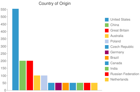
The table below shows the output from PSPP’s ‘Frequencies’ procedure. The frequencies procedure is used for analysing a single categorical variable. In this case we are comparing the different countries from which users visited the blog. From the results we can see that the majority of users were from the United States with China and the UK scoring equal second.
| Value Label | Value | Frequency | Percent | Valid Percent | Cum Percent |
|---|---|---|---|---|---|
| United States | 0 | 553 | 36.79 | 36.79 | 36.79 |
| China | 1 | 200 | 13.31 | 13.31 | 50.10 |
| Great Britain | 2 | 200 | 13.31 | 13.31 | 63.41 |
| Australia | 3 | 100 | 6.65 | 6.65 | 70.06 |
| Poland | 4 | 100 | 6.65 | 6.65 | 76.71 |
| Czech Republic | 5 | 50 | 3.33 | 3.33 | 80.04 |
| Germany | 6 | 50 | 3.33 | 3.33 | 83.37 |
| Brazil | 7 | 50 | 3.33 | 3.33 | 86.69 |
| Canada | 8 | 50 | 3.33 | 3.33 | 90.02 |
| India | 9 | 50 | 3.33 | 3.33 | 93.35 |
| Russian Federation | 10 | 50 | 3.33 | 3.33 | 96.67 |
| Netherlands | 11 | 50 | 3.33 | 3.33 | 100.00 |
| Total | 1503 | 100.0 | 100.0 | ||
Table produced by PSPP

Chart produced using the Google Visualisation API.
Next we look at the ‘Explore’ procedure, this is used for analysing metric (numerical) variables, for example, the total number of hits made by each visitor. The descriptives table shown below gives us some useful information. Firstly it indicates that the mean number of hits made to the blog was 5 (rounded from 5.05), the median was 5, the minimum value was 1 (otherwise the visit couldn’t have been recorded) and the maximum number of pages visited was 15.
| Statistic | Std. Error | |||
|---|---|---|---|---|
| Total number of hits made to the blog | Mean | 5.05 | .05 | |
| 95% Confidence Interval for Mean | Lower Bound | 4.95 | ||
| Upper Bound | 5.15 | |||
| 5% Trimmed Mean | 4.97 | |||
| Median | 5.00 | |||
| Variance | 4.25 | |||
| Std. Deviation | 2.06 | |||
| Minimum | 1.00 | |||
| Maximum | 15.00 | |||
| Range | 14.00 | |||
| Interquartile Range | 2.00 | |||
| Skewness | .65 | .06 | ||
| Kurtosis | .92 | .13 |
Table produced by PSPP
The ‘Explore’ procedure is also capable of producing percentiles analysis. We can see from the table below that up to 25% of visitors viewed at least 6 pages, 50% of users viewed up to 5 pages and 75% of visitors viewed at least 4 pages.
| Percentiles | |||||||||||
|---|---|---|---|---|---|---|---|---|---|---|---|
| 5 | 10 | 25 | 50 | 75 | 90 | 95 | 25 | 50 | 75 | ||
| Total number of hits made to the blog | HAverage | 2.00 | 3.00 | 4.00 | 5.00 | 6.00 | 8.00 | 9.00 | 4.00 | 5.00 | 6.00 |
| Tukey’s Hinges | 4.00 | 5.00 | 6.00 | 4.00 | 5.00 | 6.00 | |||||
Table produced by PSPP
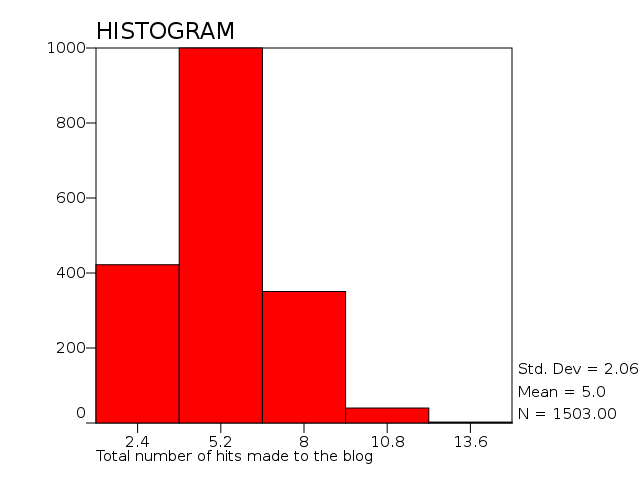
Complimenting the ‘Explore’ procedure PSPP can produce a histogram. Histograms are useful in helping us to visualise the distribution of a metric variable. Our histogram shows us that the distribution is approximately symetric. This means that we should use the mean for reporting average number of hits to the site. If the histogram was not symetric the median would give us a better value to use for the average.

Chart produced by PSPP
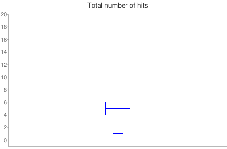
SPSS has one distinct advantage over PSPP when using the ‘Explore’ procedure. SPSS is capable of producing box plot charts. Box plots are another great way for us to visualise the distribution of a metric variable. The box plot below was produced using the Google Visualisation API with the data produced by PSPP. The top and bottom markers represent the minimum and maximum number of hits made by visitors. The box area represents the number of hits between the 25th and 75th quartiles (majority of visitors) and the line through the middle of the box represents the median.

Chart produced using the Google Visualisation API.
Hypothesis Testing
Top
As well as single variable analysis PSPP gives us the opportunity to test hypothesis. For example we might hypothesise that vistors from the United States spent more time on the blog than visitors from China because the blog is written in English. To test this we could perform an independent samples t-test using PSPP. The table below shows that the mean number of minutes spent on the site was 1.36 minutes for US visitors. Higher than Chinese visitors who spent 0.83 minutes on the site. However the ouput also shows us that the difference is not statistically significant. The significance value (highlighted in red) is higher than 0.05. We can also see that the 95% confidence level is between -0.19 and 1.25. This indicates that the difference in the entire population could be either 0.19 minutes less or 1.25 more than the mean. Unfortunately we can not draw any conclusions in this case.
| COUNTRY | N | Mean | Std. Deviation | S.E. Mean | |
|---|---|---|---|---|---|
| DURATION | United States | 553 | 1.36 | 6.44 | .27 |
| China | 200 | .83 | 3.49 | .25 |
| Levene’s Test for Equality of Variances | t-test for Equality of Means | |||||||||
|---|---|---|---|---|---|---|---|---|---|---|
| 95% Confidence Interval of the Difference | ||||||||||
| F | Sig. | t | df | Sig. (2-tailed) | Mean Difference | Std. Error Difference | Lower | Upper | ||
| DURATION | Equal variances assumed | 9.40 | .00 | 1.10 | 751.00 | .27 | .53 | .37 | -.19 | 1.25 |
| Equal variances not assumed | 1.43 | 640.76 | .15 | .53 | .37 | -.20 | 1.25 | |||
Table produced by PSPP
Looking for relationships
Top
As well as t-tests PSPP can perform regression analysis, useful when trying to identify relationships between two metric (numerical) variables. Say we suggested that as avisitor visits more pages, more data is downloaded from the server. The Correlations table below shows that the correaltion between these variables is 1.0 (highlighted in red). This indicates a very strong relationship. The coefficients table indicates that the slope is 22.8 (highlighted in blue). This indicates that on average, for every page visited, an extra 22.8kb of data was downloaded from the server. We can also see that the significance of the test is 0 (highlighted in green), as this is less than 0.05, we can conclude that the relationship is significant. As expected as page hits increase more data is downloaded from the server. Perhaps a little obvious however a test like this could help validate the data.
| Total number of hits made to the blog | Bandwidth downloaded by user (kilobytes) | ||
|---|---|---|---|
| Total number of hits made to the blog | Pearson Correlation | 1.00 | 1.00 |
| Sig. (2-tailed) | .00 | ||
| N | 1503 | 1503 | |
| Bandwidth downloaded by user (kilobytes) | Pearson Correlation | 1.00 | 1.00 |
| Sig. (2-tailed) | .00 | ||
| N | 1503 | 1503 |
| R | R Square | Adjusted R Square | Std. Error of the Estimate | |
| 1.00 | 1.00 | 1.00 | .00 |
| Sum of Squares | df | Mean Square | F | Significance | ||
|---|---|---|---|---|---|---|
| Regression | 3166653 | 1 | 3166653 | 9.7E+015 | .00 | |
| Residual | .00 | 1501 | .00 | |||
| Total | 3166653 | 1502 |
| B | Std. Error | Beta | t | Significance | ||
|---|---|---|---|---|---|---|
| (Constant) | .00 | .00 | .00 | .00 | 1.00 | |
| Total number of hits made to the blog | 22.28 | .00 | 1.00 | 98362442 | .00 | |
Table produced by PSPP
Finally, PSPP allows us to perfrom Crosstabs analysis which helps us to identify relationships between two categorical variables. In this case we have produced a crosstabs analysis, comparing the search term used to find the blog to the country of origin. One of the search terms was related to a blog post describing how to use Google’s language API. We might assume that non-english countries would be more likely to search for this as opposed to English speaking countries, as most of the webs content is in English. The crosstabs table below shows us this is the case. However a chi square test indicates that this test is not statistically significant. The significance value is greater than 0.05 (highlighted in red). Unfortunately we do not have enough information to draw any conclusions.
| Cases | ||||||
|---|---|---|---|---|---|---|
| Valid | Missing | Total | ||||
| N | Percent | N | Percent | N | Percent | |
| Search Term * Country Of Origin | 723 | 48.1% | 780 | 51.9% | 1503 | 100.0% |
| COUNTRY | |||||||||||||
|---|---|---|---|---|---|---|---|---|---|---|---|---|---|
| SEARCH | United States | China | Great Britain | Australia | Poland | Czech Republic | Germany | Brazil | Canada | India | Russian Federation | Netherlands | Total |
| as3 iterate through display objects | 33.0 | 12.0 | 11.0 | 4.0 | 4.0 | 2.0 | 2.0 | 2.0 | 2.0 | 2.0 | 2.0 | 2.0 | 78.0 |
| 12.4% | 12.5% | 11.5% | 8.3% | 8.3% | 8.3% | 8.3% | 8.3% | 8.3% | 8.3% | 8.3% | 8.3% | 10.8% | |
| curl web crawler in php | 33.0 | 12.0 | 10.0 | 6.0 | 6.0 | 3.0 | 3.0 | 3.0 | 3.0 | 3.0 | 3.0 | 3.0 | 88.0 |
| 12.4% | 12.5% | 10.4% | 12.5% | 12.5% | 12.5% | 12.5% | 12.5% | 12.5% | 12.5% | 12.5% | 12.5% | 12.2% | |
| google language api php example | 33.0 | 12.0 | 15.0 | 8.0 | 8.0 | 4.0 | 4.0 | 4.0 | 4.0 | 4.0 | 4.0 | 4.0 | 104.0 |
| 12.4% | 12.5% | 15.6% | 16.7% | 16.7% | 16.7% | 16.7% | 16.7% | 16.7% | 16.7% | 16.7% | 16.7% | 14.4% | |
| google web toolkit animation effects | 49.0 | 16.0 | 16.0 | 8.0 | 8.0 | 4.0 | 4.0 | 4.0 | 4.0 | 4.0 | 4.0 | 4.0 | 125.0 |
| 18.4% | 16.7% | 16.7% | 16.7% | 16.7% | 16.7% | 16.7% | 16.7% | 16.7% | 16.7% | 16.7% | 16.7% | 17.3% | |
| iterating dom childnodes | 31.0 | 12.0 | 12.0 | 6.0 | 6.0 | 3.0 | 3.0 | 3.0 | 3.0 | 3.0 | 3.0 | 3.0 | 88.0 |
| 11.6% | 12.5% | 12.5% | 12.5% | 12.5% | 12.5% | 12.5% | 12.5% | 12.5% | 12.5% | 12.5% | 12.5% | 12.2% | |
| kinematics in flash animation | 19.0 | 8.0 | 8.0 | 3.0 | 2.0 | 1.0 | 1.0 | 1.0 | 1.0 | 1.0 | 1.0 | 1.0 | 47.0 |
| 7.1% | 8.3% | 8.3% | 6.3% | 4.2% | 4.2% | 4.2% | 4.2% | 4.2% | 4.2% | 4.2% | 4.2% | 6.5% | |
| papervision 3d rotate cube | 33.0 | 12.0 | 12.0 | 7.0 | 8.0 | 4.0 | 4.0 | 4.0 | 4.0 | 4.0 | 4.0 | 3.0 | 99.0 |
| 12.4% | 12.5% | 12.5% | 14.6% | 16.7% | 16.7% | 16.7% | 16.7% | 16.7% | 16.7% | 16.7% | 12.5% | 13.7% | |
| zend amf example | 36.0 | 12.0 | 12.0 | 6.0 | 6.0 | 3.0 | 3.0 | 3.0 | 3.0 | 3.0 | 3.0 | 4.0 | 94.0 |
| 13.5% | 12.5% | 12.5% | 12.5% | 12.5% | 12.5% | 12.5% | 12.5% | 12.5% | 12.5% | 12.5% | 16.7% | 13.0% | |
| Total | 267.0 | 96.0 | 96.0 | 48.0 | 48.0 | 24.0 | 24.0 | 24.0 | 24.0 | 24.0 | 24.0 | 24.0 | 723.0 |
| 100.0% | 100.0% | 100.0% | 100.0% | 100.0% | 100.0% | 100.0% | 100.0% | 100.0% | 100.0% | 100.0% | 100.0% | 100.0% | |
| Statistic | Value | df | Asymp. Sig. (2-tailed) |
|---|---|---|---|
| Pearson Chi-Square | 10.29 | 77 | 1.00 |
| Likelihood Ratio | 10.49 | 77 | 1.00 |
| Linear-by-Linear Association | .35 | 1 | .55 |
| N of Valid Cases | 723 |
Table produced by PSPP